This week started with a bang. Anthropic accidentally leaked the source code for Claude Code, and within hours someone had kicked off a clean-room rewrite in Python. The internet, understandably, caught fire, and it seemed like the perfect topic to write about this week. As there were still lots of threads open, and people trying to make sense of the code base, I decided to leave it for when the dust settles (that way I could read the code base myself to draw my own conclusions before rushing into writing anything).
Fortunately, amidst the noise of Claude Code’s leak, Google Quantum AI made a release (Google featuring this newsletter again) that didn’t get the attention that I think it deserved. It was the perfect excuse to write again in this newsletter about quantum computing.
I’ve been fascinated by quantum computing since I was first introduced to it (at the time, I even wrote a patent that leveraged quantum information to reach consensus in distributed networks, but I’ll spare you the details for now). From all the new fancy technologies coming up these days, quantum computing is, to me, one of the hardest technology timelines to read. Since I’ve started following and studying closely there’s been an enormous amount of hype, a few winters, a lot of exciting progress, and no immediate use case to show off yet.
I’ve been studying the technology on the side for years, but never worked on it professionally. My only hands-on experience with the technology has been through a few Qiskit hackathons many years ago (I guess the barriers were high). I’ve been meaning to go back and get hands-on time with something like IBM’s publicly available quantum systems just to recalibrate my intuition, but I never find the time or motivation. This paper made me feel that urgency more acutely that I needed to recover this rusty skill.
The TL;DR of what Google dropped this week is a whitepaper claiming to reduce the quantum resources needed to break Bitcoin’s cryptography by roughly 20-fold. Cryptocurrencies and quantum computing… you can imagine how this topic took preference over Claude Code’s leak.
Shor’s algorithm and the hard problem underneath ECDSA
Before we get to the papers, let’s set the stage so everyone (independently of your knowledge about the space) is on the same page. This means taking a quick trip into the cryptographic primitives that currently protect every Bitcoin and Ethereum transaction.
When you sign a transaction on Bitcoin or Ethereum, you’re using a cryptographic primitive called ECDSA: the Elliptic Curve Digital Signature Algorithm. The security of ECDSA rests entirely on one hard problem: the Elliptic Curve Discrete Logarithm Problem (ECDLP). Here’s a high-level intuition of what this problem is all about.
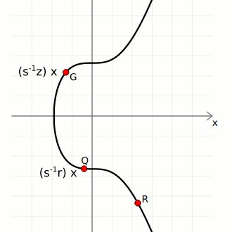
An elliptic curve over a finite field forms a specific algebraic structure: a prime-order cyclic group. You’ll see that this really matters when we discuss how it can be attacked by quantum computers. The group is generated by a single distinguished point G (the generator), and every element of the group can be written as k·G for some integer k. Your private key is that integer k. Your public key is Q = k·G, the generator point “multiplied” by your private key, where multiplication means repeatedly applying a specific point-addition rule defined by the curve’s geometry.
Given Q and G, recovering k by brute force classically (meaning with our current computing systems) requires roughly 2^128 operations on Bitcoin’s curve (secp256k1). That’s a few hundred undecillion operations, effectively the age of the universe at a billion operations per second. The problem is hard in one direction only. Computing Q from k is instant. The reverse is infeasible.This asymmetry is what cryptographers call a hard problem, and this is why they are so appealing to create cryptographic primitives out of them.
Remember my post a few months ago about complexity theory and P=NP? ?This has a lot to do with that. Cryptographic primitives are built on the assumption of hard problems complexity. Technically, ECDLP sits in NP∩co-NP, it’s not known to be NP-hard in the strict complexity-theoretic sense, and most cryptographers believe it isn’t. It isn’t known to be in P either. Another hard problem commonly used for cryptographic primitives is integer factorisation, the hard problem underlying for instance RSA, which sits in exactly the same class: NP∩co-NP, not NP-complete, not known to be efficiently solvable. Both problems are “believed hard” without being provably hard in the complexity-theoretic sense.
Both problems resist classical attacks for the same reason: no efficient algorithm has been found after decades. And here is where Shor’s famous algorithm enters the scene.
Shor’s algorithm, published in 1994, exploits the cyclic structure of the group. Rather than brute-forcing the keyspace, it uses quantum Fourier transforms and period-finding on the multiplicative structure of the group to extract k from Q in polynomial time. The precise gate complexity is approximately O(n² log n log log n) in the bit-length n of the key (often cited as O(n²) for shorthand) though the full form matters when you’re counting Toffoli gates against a hardware budget (these gates are the quantum equivalent of a controlled-controlled-NOT, used to implement AND operations reversibly. Think of it as the universal reversible gate of quantum computing, they will be important when we discuss the contributions of the papers released). For a 256-bit key, that’s tractable, if you have a sufficiently large quantum computer.
The question has always been: how large is “sufficiently large”?I think you see where I am getting at. The papers released this week seem to have changed our existing intuitions about how many qubits are needed for Shor’s algorithm to break our existing cryptography.
The two papers released
The two papers that dropped this week have made some experts reevaluate their timelines about the security of the underlying security of blockchain systems that haven’t adopted post-quantum:
The Google Quantum AI whitepaper, “Securing Elliptic Curve Cryptocurrencies against Quantum Vulnerabilities: Resource Estimates and Mitigations”. Authored by Ryan Babbush and Craig Gidney at Google Quantum AI, alongside Thiago Bergamaschi (UC Berkeley), Justin Drake from the Ethereum Foundation, and Dan Boneh from Stanford. Google also published a blog post on the responsible disclosure methodology.
Let me give you some background about some of the authors so you can frame this contribution in the state-of-the-art.. Justin Drake is one of the primary researchers at the Ethereum Foundation responsible for Ethereum’s data-availability roadmap, he was a key architect behind EIP-4844 and the KZG trusted setup ceremony. Dan Boneh is a professor of computer science at Stanford, co-director of the Stanford Security Lab, and co-author of the most widely used applied cryptography textbook in the field. His free online cryptography course has been taken by over half a million people, and some of his papers were key for the development of Filecoin (another one that hits home). Finally, Craig Gidney has been responsible for a lot of the recent progress in the intersection of quantum and AI. You can imagine the weight that claims from these people can have in their respective fields. He published a paper in May 2025 showing RSA-2048 breakable with under 1 million physical qubits, down from 20 million in his own 2019 estimate.
On the other hand, the Oratomic paper, “Shor’s algorithm is possible with as few as 10,000 reconfigurable atomic qubits”, comes from Oratomic, a neutral-atom quantum computing company out of Pasadena, with John Preskill (Caltech) and Dolev Bluvstein as co-authors. Crucially, the Google whitepaper cites the Oratomic circuits as its own input, the two papers are cross-linked and share the same circuit design.
The papers present two circuit variants for attacking secp256k1:
Circuit 1: ≤1,200 logical qubits, ≤90 million Toffoli gates
Circuit 2: ≤1,450 logical qubits, ≤70 million Toffoli gates
Translated to physical hardware using surface codes on a superconducting architecture (planar degree-4 connectivity, consistent with Google’s Willow-class chips): fewer than 500,000 physical qubits. The previous best estimate, Litinski (2023), put this at roughly 9 million physical qubits. Google just moved that needle by nearly 20-fold.
That reduction didn’t come from a hardware breakthrough, it came from a better circuit. Running Shor’s on ECDLP isn’t just “run the algorithm” (this is somethign I learnt the hard way the first time I was tinkering with Qiskit and IBMs quantum computers). The core computation is elliptic curve point multiplication, computing k·G for arithmetic on secp256k1, which Shor’s algorithm needs to evaluate in quantum superposition as part of its period-finding routine. That means implementing modular arithmetic (specifically Montgomery multiplication, the standard technique for efficient modular operations) entirely in reversible quantum gates.
Every classical arithmetic operation has to be “uncomputed” after use to avoid accumulating garbage qubits that would corrupt the superposition. The dominant cost is Toffoli Gates and there are hundreds of millions of them in a naively constructed circuit.
Prior work optimised either qubit count or gate count, but not both simultaneously. The relevant figure of merit for real hardware is spacetime volume, i.e. the product of qubits × gates × cycle time, because that’s what determines wall-clock runtime on an actual machine.
Google’s contribution is a circuit that achieves the best spacetime volume ever published for ECDLP-256, through two main improvements. First, they applied improved windowing to Montgomery multiplication: rather than processing one bit of the scalar at a time, they process wider windows, amortising the Toffoli cost across more bits per round, reducing the total gate count substantially.
Second, they revised the T-state factory overhead: magic state distillation (the process for producing the high-fidelity ancilla states that Toffoli gates consume) is the dominant physical qubit cost in any surface-code implementation, and prior estimates were conservative. More careful accounting of distillation factory layout and scheduling cut the physical qubit estimate significantly. The combination brought the spacetime volume down far enough to halve the physical qubit requirement relative to Litinski 2023, and Litinski 2023 had already improved substantially on everything before it.
But before going any further I think is worth stressing the distinction between logical and physical qubits and why this matters. Theoretical qubits are what algorithms assume, perfect, noiseless two-state quantum systems. Logical qubits are error-corrected abstractions built from many physical qubits using a quantum error-correcting code (typically a surface code, I have to admit that loving information theory this field of error-corrected qubits is one that I am fascinated about. I actually leverage some of these error-corrected algorithms for my patent).
Physical qubits are the actual noisy hardware. Today’s devices operate at error rates around 10^-3 per gate, which means you need roughly 1,000 physical qubits to sustain one reliable logical qubit. The overhead varies by architecture and target error rate, but it’s the dominant cost in any near-term hardware plan.
To put the current state in perspective: Google’s Willow chip has 105 physical qubits. IBM’s Condor processor reached 1,121 qubits in late 2023, the largest superconducting qubit count to date, though not all at useful error rates. The gap between today and 500,000 error-corrected qubits is still enormous. But the conceptual threshold has moved, and it’s moved faster than almost anyone expected.
The two papers cover different hardware architectures, and the distinction matters. Superconducting qubits, the technology behind Google Willow and IBM’s quantum systems, encode quantum information in tiny circuits cooled near absolute zero (i.e close to 0 Kelvins), where electrical resistance vanishes and quantum effects dominate. Gate operations run in nanoseconds to microseconds. Neutral-atom architectures, like those used by Oratomic, trap individual atoms using focused laser beams and manipulate their quantum states optically. They achieve extremely long coherence times and flexible qubit connectivity, but gate operations are around 1000x slower). Ion trap systems (IonQ, Quantinuum) work on similar principles: individual ions levitated in electromagnetic fields and controlled with lasers. IonQ’s Forte system currently achieves around 29 “algorithmic qubits”, roughly the effective logical qubit count after accounting for noise. The Oratomic team reported 6,100 coherent atomic qubits trapped, with fault-tolerant operations demonstrated below the error threshold on around 500 qubits.
The Oratomic result is the more striking one in raw qubit count: the same computation runs with as few as 10,000–26,000 qubits on neutral-atom hardware. The catch: at current clock speeds (around 1ms/cycle), runtime is close to 10 days, not minutes. That limits the attack to at-rest targets, long-dormant wallets that have been sitting on-chain for years, not live transaction interception.
That clock speed difference is one of the genuinely novel framings in these papers. Superconducting hardware runs gate cycles in microseconds; neutral atoms and ion traps are 100–1,000x slower. This determines which kind of attack is feasible. The papers define three categories: on-spend (race Bitcoin’s block clock before the transaction confirms), at-rest (target publicly exposed keys on dormant wallets), and on-setup (recover secrets from one-time cryptographic ceremonies like KZG). Fast-clock architectures enable on-spend. Slow-clock ones are limited to the other two.
The ZKP disclosure 😱
Here’s the part that really blew my mind about Google’s whitepaper (and that I think justifies even more having Justing Drake and than Dan Boneh around for the paper). Google did not publish the attack circuits. Instead, they published a zero-knowledge proof that the circuits work.
The attack circuit, a sequence of quantum gate operations implementing Shor’s algorithm for secp256k1, was written as an ordinary Rust code using a quantum circuit library that models qubits, gates (Hadamard, CNOT, Toffoli, phase rotation), and multi-qubit arithmetic operations. The program encodes the Montgomery modular multiplication routine at the core of the elliptic curve group arithmetic, the quantum Fourier transform used for period extraction, and the bookkeeping that wires those components into a complete Shor’s instance for ECDLP-256. The circuit itself is a classical description of a quantum computation, a directed graph of gate operations to be executed on hardware. It’s the blueprint, not the machine. (sidenote: the circuit of the image is the classical implementation of Shor’s algorithm for those of you that haven’t seen one ever).
That Rust program was then fed into SP1, a zero-knowledge virtual machine built by Succinct Labs which targets the RISC-V architecture. For those unfamiliar with ZK-VMs, SP1 compiles Rust to RISC-V bytecode (using the standard RISC-V target), and then generates a cryptographic proof, specifically a STARK-based proof, that a given RISC-V program was executed correctly on specific inputs and produced a specific output. You get a proof of correct execution without anyone needing to see the program or the inputs.
In this case: Google ran the circuit program against 9,000 randomly sampled secp256k1 input points, verified that the circuit correctly performs the elliptic curve operations it claims to, and had SP1 generate a proof of that execution. The SHA-256 hash of the circuit was committed publicly so anyone can verify they’re talking about the same circuit. The SP1 proof attests: “this hash corresponds to a program that, when run on these inputs, produces these outputs consistently with a correct Shor’s implementation for ECDLP-256.”
The inner SP1 proof is a STARK. STARKs have no trusted setup, but they’re large, hundreds of kilobytes to megabytes. So SP1 wraps the STARK in an outer Groth16 SNARK. Groth16 takes the STARK proof as a statement to be proved and generates a compact proof of it: roughly 200 bytes, regardless of the complexity of the original computation. The final artefact, code and proof, sits on Zenodo. Anyone can download it and verify Groth16’s 200-byte proof in milliseconds, without ever seeing the attack circuit.
What this means practically: the existence and correctness of the attack is publicly verifiable. The attack tool itself is not.
This is a genuinely new move in responsible disclosure. The standard practice for software vulnerabilities is to notify the vendor, wait a window, then publish. But there’s no vendor to notify here, no patch to deploy in 90 days. So Google found a different answer: prove the result is real, withhold the exploit.
Here’s where it gets funny, or uncomfortable, depending on your perspective. Groth16 is itself an elliptic curve construction. It operates over BN254, a pairing-friendly curve distinct from secp256k1, but it is still fundamentally an elliptic curve scheme. The pairings that make Groth16 work rely on the same class of hard problems, discrete logarithms on elliptic curves, that Shor’s algorithm can break. So Google used a cryptographic primitive that is also eventually threatened by sufficiently powerful quantum computers to prove the existence of the circuit that threatens elliptic curve cryptography. If CRQCs (Cryptographically Relevant Quantum Computers, the term the whitepaper uses for machines capable of running these attacks) ever arrive at scale, Groth16 and the broader ZKP ecosystem go down with the rest.
I don’t know if that’s elegant or just funny. Probably both.
But what is even crazier to me is that this could become eventually the standard model for future research and proprietary algorithms, where companies and researchers can show that “their algorithms do what they claim to be doing” without leaking anything about its underlying implementation. That’s enough for a post of itself. I’ve been saying it for a while but ZKP primitives can have immediate use outside of blockchain networks and web3.
Post-quantum cryptography: what exists, what migration looks like
To understand why certain cryptographic schemes survive a quantum computer and others don’t, we need to understand why Shor’s algorithm works in the first place.
Shor’s algorithm is a period-finding machine. It exploits the fact that ECDLP and integer factorisation both reduce to finding the period of a function defined over a cyclic algebraic group. Quantum Fourier transforms make period-finding tractable on cyclic structures, and that’s the attack. The quantum speedup isn’t general; it’s specific to problems with this periodic structure. If you pick a hard problem that doesn’t have it, Shor’s doesn’t help.
That’s exactly what post-quantum cryptography does.
Lattice problems, specifically the Shortest Vector Problem (SVP) and its structured variant, Module Learning With Errors (MLWE), ask you to find the shortest non-zero vector in a high-dimensional lattice, or to distinguish a structured equation system from a random one. Neither problem has a cyclic group structure Shor’s can exploit. The best known quantum algorithm for SVP offers only a polynomial speedup over classical approaches, not the exponential gap that Shor’s gives against ECDLP.
SVP is NP-hard in the worst case, and lattice cryptography has an elegant property: worst-case hardness reduces to average-case hardness, which makes the security proofs unusually strong. The specific structured variants used in practice (MLWE, MSIS) sit slightly off the worst-case problem, so ongoing cryptanalysis remains active, but no quantum attack comes close to breaking them.
Hash-based problems rest on collision resistance alone. There is no algebraic structure, no group, no lattice. If SHA-256 or SHAKE-256 resist collision attacks, and there’s no known quantum or classical attack that breaks them, the scheme is secure. Grover’s algorithm gives a quadratic speedup for unstructured search, which halves the effective security level (256-bit security becomes 128-bit), but doubling the output size restores it. That’s a parameter choice, not a structural break.
Code-based problems, specifically the Syndrome Decoding Problem, ask you to find a codeword in a random linear error-correcting code given a corrupted version. Berlekamp showed in 1978 that SDP is NP-complete in the worst case. No quantum speedup beyond polynomial is known. The cost has historically been large key sizes (around 1MB for McEliece-based schemes), but newer constructions have reduced this substantially.
The NIST post-quantum standards (i.e. list of post-quantum standards so far accepted by NIST) are a portfolio of bets across those three problem families:
ML-KEM (FIPS 203), key encapsulation, formerly CRYSTALS-Kyber. Lattice-based (MLWE). FIPS-finalised, production-ready.
ML-DSA / Dilithium (FIPS 204), digital signatures. Lattice-based (MLWE/MSIS). Signature size: ~2.5KB. FIPS-finalised, production-ready.
SLH-DSA / SPHINCS+ (FIPS 205), stateless hash-based signatures. Signature size: ~8KB. FIPS-finalised. Heavy but the most conservative security assumption available.
HQC, selected March 2025 as fifth KEM, full standard expected 2027. Code-based (syndrome decoding). Smaller keys than McEliece.
And why not migrate immediately to these primitives. The main issue rests in the size of the keys, that can mean breaking a lot of assumptions in some systems (including blockchain networks). Post-quantum keys can be 100-fold larger than existing ECDSA and even RSA keys.
Has the timeline really changed?
What about all of this claims and the statement in Google’s paper about this discovery making them “reevaluate” current quantum supremacy timelines? My immediate answer would be, “who knows?”
Here’s one thing that I think some people may be missing when reading this results: the dramatic reduction in resource counts is real, but the practical problem is not about how many qubits you need on paper. It’s about whether you can build qubits good enough to make those counts mean anything.
The Google whitepaper assumes a physical gate error rate of 10^ 3 sustained uniformly across all qubits. That’s the modelling assumption. Where is hardware today?
The state of the art, as of 2024, is two-qubit gate fidelity of ~99.9%, which is exactly 10^ -3. Multiple groups have now reported this number, including Google with Willow. So you might conclude the assumption is already met. Scott Aaronson (you probably remember him as being my favourite computer scientist alive :) ), who has been tracking this more carefully than most, made exactly this point in September 2024:
“Within the past year, multiple groups have reported 99.9% [two-qubit gate fidelity]. I’m now more optimistic than I’ve ever been that, if things continue at the current rate, either there are useful fault-tolerant QCs in the next decade, or else something surprising happens to stop that.”
But he also noted that 99.99%, a full order of magnitude better, is what you really need for sustained fault-tolerant operation where error correction delivers a net gain rather than just breaking even. That threshold hasn’t been reached.
There’s a version of the coverage that reads these papers as evidence the timeline itself has shortened. I don’t think that’s right, and the distinction matters. What these papers changed is the target: the number of qubits and gates required on paper to run the attack. What they didn’t change is the distance to that target, which is determined entirely by hardware, and hardware hadn’t moved much this past month. The Willow chip had the same error rates the day after the whitepaper dropped as it did the day before. A more efficient attack circuit doesn’t build better qubits. It lowers the bar you need to clear, but if you can’t clear the bar yet, lowering it isn’t the same as getting closer.
More critically: those fidelity numbers are measured on the best qubit pairs on a 100-qubit chip under carefully optimised conditions. Nobody has demonstrated 99.9% gate fidelity sustained uniformly across a million physical qubits.
Google’s own Willow error correction paper, the paper that demonstrated below-threshold surface code performance for the first time, achieved that milestone on 101 physical qubits. The target for a cryptographically relevant attack is somewhere between 500,000 and 1 million. The Willow paper itself notes that logical performance is limited by rare correlated error events, roughly once per hour, that fall outside the standard noise model fault-tolerance proofs assume. At million-qubit scale, the frequency and character of those events is unknown.
Then there’s inter-chip communication. Gidney’s estimates assume a planar grid of qubits with nearest-neighbour connectivity. At the million-qubit scale, that means stitching together many chips into a coherent quantum system, something that has not been demonstrated anywhere. Aaronson again: “eventually you’ll need communication of qubits between chips, which has yet to be demonstrated.”
There’s still a sentence near the end of the whitepaper that I think frames the risk correctly:
“It is conceivable that the existence of early CRQCs may first be detected on the blockchain rather than announced.”
That’s the authors acknowledging a tail scenario the “Nassim Taleb-way”: a nation-state or well-funded private effort builds this quietly, and the first public evidence of success is unexplained large wallet drains on-chain (my good friend Marko Vukolic always said that Bitcoin and Satoshi’s wallet was the biggest quantum computing bounty available, so this claim adds up).
So the honest position is: the resource count dropped dramatically, and that matters. But the real question for the timeline isn’t how many qubits you need on paper, it’s whether anyone can build a million qubits that are actually good enough.
We’ll have to wait and see… Until next week!